Blog_AUS_Bushfires_19_20

AUSTRALIA'S BUSHFIRES

AUSTRALIA'S BUSHFIRES: 2019/2020 ANALYSED WITH NASA SATELLITE  DATA
by Ditty April 2020
Keywords: Bushfires, Australia, NASA, Geo Spacial Analysis


Introduction - What is going on 
Last November (2019) until February (2020) I was traveling from The Netherlands to the lovely country down under, Australia. The moment the airplane touched down on Australian soil - I felt this was going to be great place to spend some time! As an avid traveller different countries tend to set-off different senses. For me the likes of Iceland, Sweden and Japan have always been of particular intrest. As these countries balance an impressive (and almost overwhelming) nature with great city experiences. So I was bound for a treat down under! Or as the kindest barista in Melbourne's CBD said: "You've come to there right place - aye mate. We’ve got heaps of ’em!" 

From Observation to Research Area
After unwinding a bit from a long journey and finally getting over my over my jetlag - I decided to travel to Sydney and from there 'play it by ear' in terms of travelling to nature's finest. On top of the list was a hike in the blue mountains. Just to give you a sense of direction and the magnitude of the national park (and the parks nearby) you can find the map below. If you want to know more about park you should definitely check the NSW National Parks and Wildlife Service website

At the same time of planning my trips I also started noticing (it was actually hard not to) that something was going on in Australia. There were days that there was a 'sepia filters-ish' tone visible and an intensive smell of smoke was noticeable. For that reason I started to investigate a bit more what was actually going on. I felt somewhat confused noticing that life in the big cities was continuing while other parts were burning. And there you have it: my first introduction to Bushfires. The topic of this research.

Research Question - what better to understand
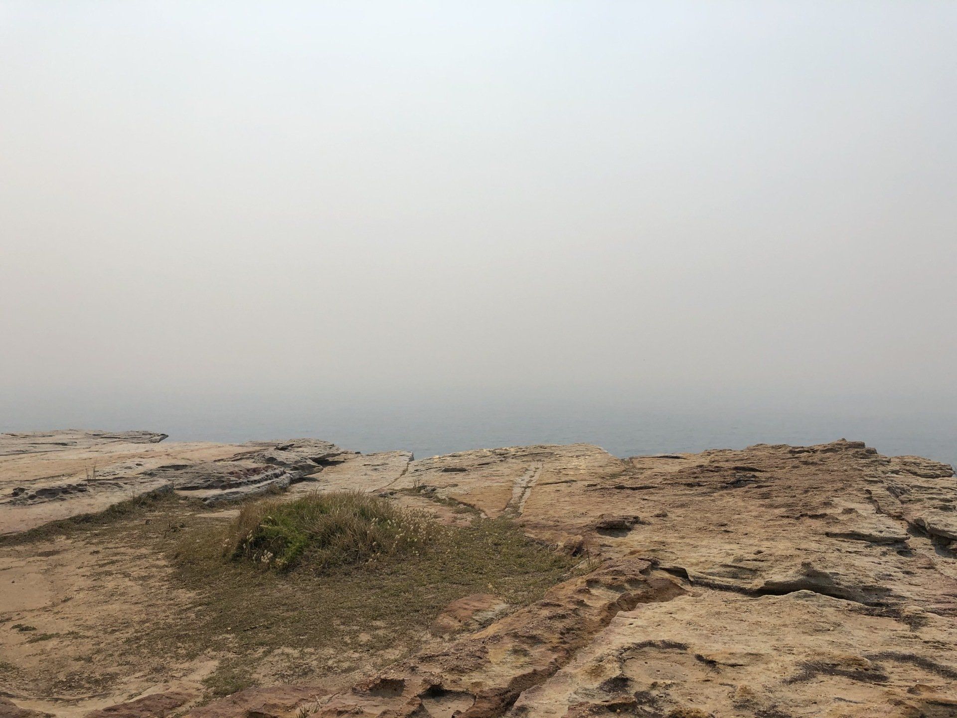
When further investigating this phenomenon off course al lot of information and opinions can be founds in the media. As it's never been in my character to hold an opinion agains someone, but is in my nature to form one based of facts. Hence, I decided to analyse this phenomenon properly when back in The Netherlands.  At that time I formed a clear sense of what I was going to study and formulated the following research question:

1. How did the wild fires develop in Australia during the bushfire season of 2019/2020?


Data collection & manipulation
Over the years I have developed a particular interest in geo-spatial analysis. With the use of R (language and environment for statistical computing and graphics) I will be using data science technique and methods like descriptive statistics, geo-spatial analysis and multi-variate analysisThe insights can be used to track and analyse how the bushfires developed across Australia, and possible give insight towards fire fighting capacity decisions. Where, I am well aware that my knowledge is relatively limited compared to local (Australian) knowledge. Hopefully this research helps as a first introduction in explaining the bushfires for people less familiar with this phenomenon. Similar to my situation, before travelling to Australia.  

Before starting to analyse the bushfire data. We need to find out how to get acces to this data. After some preliminary desk research I foresaw two data science techniques for collecting the data. 

  1. Web-scraping the data from sources like wikipedia. 
  2. Using NASA's satellite data with heat detection algorithm

An easy choice
Webscraping: although I'am a partizan of fast prototyping in my code and initially pay less attention to re-usability of it (I usually do that after finalising the project) web scraping as - I once again discovered in my Corona related posts-  can be a a time consuming and ordeal experience. Digging trough the source HTML of sites and transforming the data into workable tables and objects in your RStudio can get messy. And then....NASA satellite data! As somewhat of a geek (or actually - full on one) I got very excited about the possibility of working with Satellite data from NASA!. (you guess which one  - were going to use in research) . Yup, NASA data - it is!


Meta Data: what data is available 
The further I got in the NASA documentation - I started realising that utilising this option might be achievable. Where, as with every post I take into account that readers do not need to have deep understanding about statistical or data science concepts. 

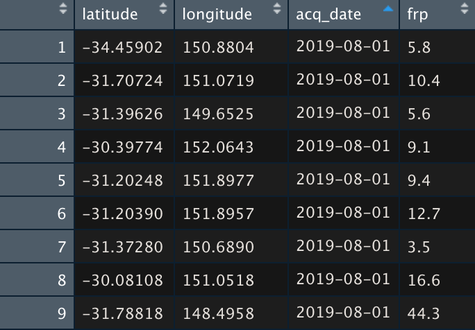
The data can be found on the NASA's active fire site. A quick scan of this page provides us the information that data from the satellite is detected across the globe in the following regions. 

  1. Alaska
  2. Conterminous US and Hawaii
  3. Central America
  4. South America
  5. Europe
  6. Northern and Central Africa
  7. Southern Africa
  8. Russia and Asia
  9. South Asia
  10. South East Asia
  11. Australia and New Zealand

Limitation / Scoping
For this analysis we are interested in the ' Australia and New Sealand' data. (Keep in mind for future research, how great is - knowing that the data is also available for all other regions).


Evaluating Data Sources - a step back to get the full picture
While reading through the site I also found that NASA uses different sensors (instruments) and algorithms onboard different satellites for (fire) detection purposes, being VIRSS and MODIS. 

Without reproducing the entire contents of both source documents, I will try to give a short(er) and simplified summary. I hope I succeed in that. Please note that I'am literally not a (space)rocket scientist, but am completely fascinated by trying to make sense of the satellites, the instruments onboard and the data they produce.

So, let's have a closer look at the two!


The Visible Infrared Imaging Radiometer Suite (VIIRS) instrument is an instrument on board of the Joint Polar Satellite System (JPSS)
"It collects visible and infrared imagery and global observations of the land, atmosphere, cryosphere and oceans".(https://www.jpss.noaa.gov/mission_and_instruments.html, 2020 April)

Together with the other instruments it collects data about "atmospheric, terrestrial and oceanic conditions, including sea and land surface temperatures, vegetation, clouds, rainfall, snow and ice cover, fire locations and smoke plumes, atmospheric temperature, water vapor and ozone" (https://www.jpss.noaa.gov/mission_and_instruments.html, 2020 April)

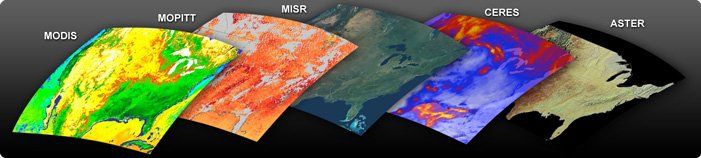
The other instruments (next to VIIRS) consist of: 

ATM: The Advanced Technology Microwave Sounder (ATMS) instrument is a next generation cross-track microwave sounder that of special interest for '...weather and climate related topics  based on atmospheric temperature and moisture profiles'.(https://www.jpss.noaa.gov/mission_and_instruments.html, 2020 April)

CERES: Clouds and the Earth's Radiant Energy System
special interest for studying "...solar energy reflected by Earth, the heat the planet emits, and the role of clouds in that process". (https://www.jpss.noaa.gov/mission_and_instruments.html, 2020 April)

CrIS: Cross-track Infrared Sounder 
special interest for studying: "...detailed atmospheric temperature and moisture observations for weather and climate applications."
(https://www.jpss.noaa.gov/mission_and_instruments.html, 2020 April)

OMPS: Ozone Mapping and Profiler Suite 
special interest for investigating "the health of the ozone layer and measures the concentration of ozone in the Earth's atmosphere".
(https://www.jpss.noaa.gov/mission_and_instruments.html, 2020 April)

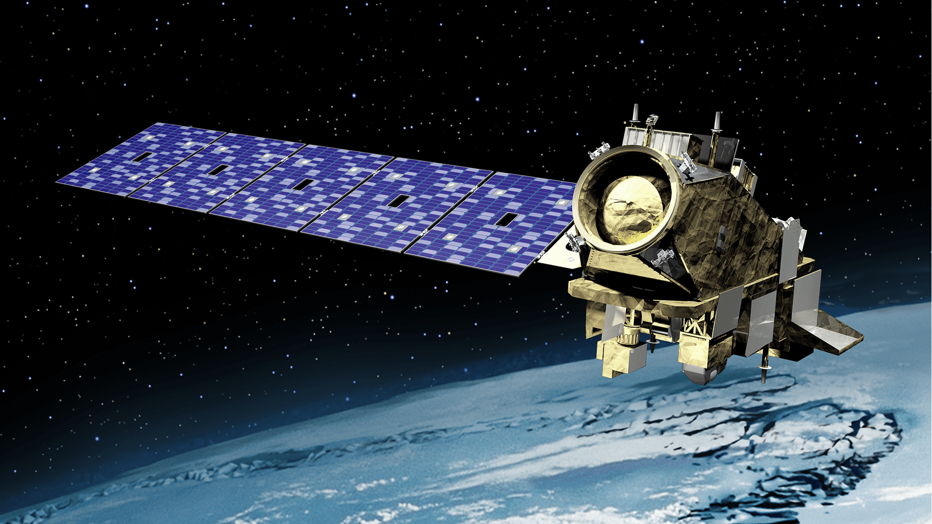
Below you see an image of the Joint Polar Satellite System (JPSS). 
Taken from (https://www.jpss.noaa.gov/satellite_gallery.html#gallery-14, 2020 April)
*please note that I couldn't find anything on sharing the image. Hoping its ok to share with source. If not will be more than willing to remove it from here
The Moderate Resolution Imaging Spectroradiometer (MODIS) instrument on the Terra Satellite has a suite of instruments onboard. It is able to track a wide range of observations. From "distribution of cloud cover to identifying tiny liquid or solid particles in the atmosphere" (https://terra.nasa.gov/about/terra-instruments/modis, 2020 April)

Although the satellite was launched in 1999  the suite of instruments are still (or in particular in the current climate change discussions) extremely relevant. Where, according to the site "Terra explores the connections between Earth's atmosphere, land, snow and ice, ocean, and energy balance to understand Earth's climate and climate change and to map the impact of human activity and natural disasters on communities and ecosystems" (https://terra.nasa.gov , 2020, April).

The other instruments (next to MODIS) consist of: 

MOPITT: Measurement of Pollution in the Troposphere 
of special interest for investigating release of carbon monoxide into the atmosphere 

MISR: Multi-angle Imaging Spectro Radiometer.
special interest for studying claret change from the perspective of the amount of sunlight different part of the world get

CERES: Clouds and the Earth’s Radiant Energy System
special interest to assess the earths net energy from the perspective of clouds by capturing the earth's 'heat energy' and 'reflected energy'.

ASTER: Advanced Spaceborne Thermal Emission and Reflection Radiometer
special interest for creating detailed maps of land surface from the perspective of the use by infrared, red, and green wavelengths of light.

As can be seen in the image below are are the different continuous layers the Terra instruments provide. 
*please note that I couldn't find anything on sharing the image. Hoping its ok to share with source. If not will be more than willing to remove it from here
Data evaluation
So now that we have investigated the different data sources. We can start with the data processing (also referred to as data manipulation). However as both NASA instruments (VIRRS vs. MODIS) show similarities in measurement units a choice needs to be made towards which data source fits our analysis best. 

In daily practice this is usually done by running some data quality / validation checks on both sources. During these processes computerised checks are performed to check the data quality. E.g. missing data or outliers / anomalies

In our case the choice is somewhat easier as based on a the level of granularity the lenses on the VIRRS instrument are stronger than those on the MODIS. As can be read in a comparison of both instruments by Guenther,  DeLuccia et all., 2011 https://www.star.nesdis.noaa.gov/jpss/documents/meetings/2011/AMS_Seattle_2011/Poster/A-TRAIN%20%20Perf%20Cont%20%20MODIS%20Observa%20-%20Guenther%20-%20WPNB.pdf, 2020, April)

Concluding that for this analysis we will solely focus on the VIIRS data from Kaggle.

Assumptions
As the posts here always have a learning component in it - for this analysis I wanted to add a different perspective to geo spacial analysis. In a previous post about the spread of the Corona virus in China I used a technique - based on date/time stamps and location coordinates to create an interactive time-lapse how the spread developed across China in the early stages of the epidemic. A similar approach would be fairly straightforward to accomplish.in this research. 

However after some feedback from colleagues and friends, where they pointed out that such animations do give a 'nice-to-have' general impression, it remains a challenge to gain deeper insights due to the 'animated' component. (things jumping up and down the entire time). 

For this reason I wanted to have a different approach in this analysis, and thus decides to work with heat maps and during the analysis process underfund what the best alternative would be for moving animations and provide sufficient information for readers. 

Managerial Implication 

In general I like the iterative approach mentioned above where you don't have a full detailed picture on what the outcome is going to be. For me it always works best to start and find out along the way. Where a possible conclusion might also be that we need to alter the research question or draw the conclusion that under the current circumstances it might not be a fruitful endeavour to pursue this analysis. The reasons why I am stressing this, and it might be a small sidestep. I see this happen a lot in data science initiatives going wrong. Mainly because there is a mis-match between (innovation) objectives and (data science) initiatives. Let me try and explain.

I am a firm believer of balanced data science initiatives in terms of 'experimentation vs optimisation' across different horizons of growth (McKinsey’s Three Horizons of Growth Model) Meaning that for different horizons you need different granularity in requirements. Different team structures and different managerial tools. So we need to answer questions as what is out objective? (experimentation or optimisation). Who do we need? (explorers or optimisers etc).How are we going to manage the process (Agile , waterfall etc.)

Although I truly believe in an agile midset to fully utilise data science within an organisation I sometimes observe a challenge within (cross) functional departments when SCRUM mythology is implemented too rigid. The horizons mentioned below are a synthesis of my experience and the McKinsey’s Three Horizons of Growth Model. Where a key constraint of the initial McKinsey’s Model is that it was implemented with increasing delivery times across increasing innovative horizons. As Steve Blank in his article in HBR rightfully pointed out - is that this assumption is no longer valid. As disruptive competition might force major innovation (related to traditional level three) under tighter time constraints.

Horizons of Growth 
  1. daily operational processen: focussing on automation of data science products eg implementing of predictive modelling (my humble view)
  2. horizon one innovation: focussing on '..core capabilities in the short-term'. (Blank, 2019)
  3. horizon two innovation: focussing on '..core capabilities to new customers, markets, or targets'. (Blank, 2019)
  4. horizon three innovation: focussing on '..new capabilities and new business to take advantage of or respond to disruptive opportunities or to counter disruption'. (Blank, 2019)


Let's get started!
Now let's get started with analysing the data. To answer our research question: "How did the wild fires develop in Australia during the bushfire season of 2019/2020?" - we will need to have a closer look at the available features in the data set. After reading the files into our R analysis environment the image below illustrates the features and definitions (also referred to as meta data) that are in our dataset.
Meta Data
  • Longitude: Fire pixel latitude
  • Latitude: Fire pixel Latitude
  • Acq_date Detection date
  • FRP: Fire Radiative Power (MW) sub-pixel
Preliminary feature analysis 
Now that we know which features are available we can perform a preliminary analysis on the data set. As can be seen in the image above the data set provides daily values for map coordinates and the detected fire intensity. Implying we have a daily picture of the entire Australian and New Zealand are with all the fires. Although this is very valuable information from a statistical / analytical perspective it might be interesting to create additional features - that help provide deeper insights about the data set. In statistics a key concepts deals with distribution of observations. E.g. how many times does a particular value occur in our data set.  

In this case I was particularly interested in the development of the FRP over time and how many times certain FRP values occurs. For this we can use data reduction technique by adding decile classes based on the FRP values and plotting the values in a box plot. Say what? Let me explain. By dividing the data set into equal amount of observation, meaning that the data set now has ten categories ranging from 1 to 10 -  and sorting the data set on the value we want to analyse, in this case FRP. We can (then) analyse each category in more detail and create a better understanding on the distribution and the internal decile distribution. Why would you want to do this? As I would expect this to gives us hints towards peak days and the corresponding values FRP. Please note that it is not a method set in stone, all we're aiming for here is to create a better (statistical understanding) on what were analysing. The images show how the FRP developed over time and and how the distribution of FRP values. In practice this sometimes means looking at your data from different angles. 
Daily FRP Vales over time
In this figure you can observe daily (total) FRP vales for all available coordinates developed over time. Meaning that from the data set all individual coordinate - values are summed in order to calculate a single value per day. Where the average FRP value is represented by the blue dotted line. As can be seen there are peaks with extreme high values end December and early January.
FRP Deciles 
In this figure you can see how the distribution of the data set looks when dividing into 10 equal categories. After inspecting the box plot in more detail, -because it looked different that I would have expected- it gave me hints that with the perspective of using deciles I was using the wrong data perspective. As I previously referred to. Why? As can be seen all 10 categories are quite similar except the categorie 10. This is something I wasn't expecting, and thus needing to further analyse what's going on here.  Only then realising that this plot is very logical as on a daily basis we have the same amount of observations, and thus might just be categorising daily distributions.  
Although it did not provide the expected insights I think it is important to mentions as I think learning from other's mistakes (in this case my mis-interpretation of the provided data) can be very useful. Summarising, no deciles for us!
Further analysis 
Loosing some time with investigating why my decile approach didn't work I then quickly turned to going back to drawing board by asking myself what I wanted answer and show. I realised that on a daily basis I wanted to provide a tool that could help in diversifying fire reaction responses. With this I mean that it might be favourable to have different fire response reactions when dealing with small(er) fires compared to larger fires. As by looking at the smaller fires this might give us insights if these could develop into bigger fires. E.g. by merging with other fires. Where the bigger fires would demand more immediate response. From a data perspective this approach is fairly straightforward to implement. As we would classify low intensity fires and high intensity fires, based on the daily:  (a) minimum FPR value, (b) maximal FPR value, (c) the average FPR value and (d) standard deviation in FPR value. The latter (standard deviation) gives us insights of how the spread of the FPR value is. 

The figures below show how an feature is added to the data set in order to identify the lowest daily FPR location and the highest daily FPR.
Creating the maps
Now that the data set has been dived into 2 sets, namely a low risk set and and high risk set we can plot this data on heat-maps. Where on a daily basis you are able to see low FRP value locations and high FRP value locations. The first illustrates ow FRP's and the second high FRP value locations. Please note that these are only the images from my R environment. 
Conclusion
In this post I tried to give more insights on how the bushfires developed in Australis by analysing NASA satellite data provided by the VIIRS instrument on board of the Joint Polar Sateliite System. 

Here we presented heat maps based in the intensity of the Fire Radiative Power picked up by VIIRS. My objective was to provide more insights on how the fires developed with relative small amounts of code, and laying the basis for future research focussing more on predictability. In this stage I hypothesised a diversified fire response approach based on the daily: (a) minimum FPR value, (b) maximal FPR value, (c) the average FPR value and (d) standard deviation in FPR value in terms of identifying low and high risk areas.

Additional to that I also made a short sidestep synthesising this analysis and how data science initiatives can be organised in organisations according to research objectives focussing on innovation horizons.
Future Research
An interesting follow-up study (usually also follows the analytical maturity model) would be to incorporate other datascores  into our model. In our research we merely classified low and high risk based on FPR vales. Where weather data (wind, temperature etc.) can contribute to better classification And in a later stage prediction of FPR vales.

eg weather data. This can contribute to creating a predictive model with the uses of supervised and unsupervised machine leaning techniques. Hence, we could start with an attempt to build a model that predicts FRP values

With the creation of such a model a further contribution can be made (a) diversified fire responses and (b) in the allocation of fire fighter capacity across geographical locations. 
Hope you enjoyed reading! 

All the best,

Ditty

Ditty Menon, The Data Artists, Ditty

About the Author: Ditty Menon

Founder of The Data Artists, The Data Artists Music and Nederland Wordt Duurzaam


Erasmus University Rotterdam Alumni with 12 years of experience in Data Science / Analytics / Digital. Passionate about incorparating data into all aspects of life & (more recent) using data for a sustainable world.


Radom facts:

Starts his day with a flat white or caffe latte and the financial times podcast.

Broke his glasses when walking into a lamppost while thinking of a coding issue

Loves Serendipity

Share by: